Keeping it Cool

The Habitable Zone Planet Finder, being an infrared spectrograph, must be kept from being saturated by infrared radiation emitted from the surroundings. This can be done by keeping the instrument extremely cold–180K, to be precise. It must be kept at that fixed temperature to milli-Kelvin precision, as any variations will increase RV measurement errors. How do we achieve this? Take a look at the figure below.

The HPF radiation shield – a vacuum chamber which contains the instrument optics – along with the liquid nitrogen (LN2) tank are both covered in MLI blankets for thermal insulation, and along with the copper thermal straps and the heater panels, they are responsible for keeping HPF at 180K with milli-Kelvin precision.

We need to consider four things:

Cooling agent – We use liquid nitrogen (LN2) to cool the instrument. The LN2 tank is at a fixed temperature of 77K at atmospheric pressure.
Conductive paths to the vacuum chamber – To cool down the radiation shield, we connect it with the LN2 tank with highly thermally conductive copper thermal straps. The straps need to be sized properly to not draw too much heat (resulting in a too cold chamber), nor too little heat (chamber too warm) from the vacuum chamber over long periods of time. The copper straps are sized to cool the vacuum chamber down to temperatures slightly cooler (around 160K – 170K) than the 180K end temperature goal.
Heater Panels – These panels heat the over-cooled radiation shield to the 180K temperature goal, and at the same time give us the milli-Kelvin precision required.
Thermal Insulation – Lastly, all of the above components are kept under high vacuum, and are all covered with Multi-Layer Insulation blankets (MLI–commonly used for space probes!), to provide effective thermal insulation from the outside world.

Radiative equilibrium

The radiation shield is on one hand being heated up by the radiation from the surroundings (at room temperature) and by the heater panels, and being cooled down from the copper thermal straps on the other. At equilibrium we can write:

$H_{\mathrm{rad}}+H_{\mathrm{Heaters}}=H_{\mathrm{Cu}}$

where $H_{\mathrm{rad}}, H_{\mathrm{Heaters}}, H_{\mathrm{Cu}}$ , denote the heat current from the net incoming radiation, the heaters, and the copper straps, respectively. Each of these factors are discussed below; this discussion might be a bit on the technical side – if so, feel free to skip to the bottom to see pictures from the copper thermal strap and heater panel preparation.

I. Incoming radiation

First off, let’s consider the incoming radiation. All objects, regardless of their temperature, emit energy in the form of electromagnetic radiation: the warmth of the Sun and glowing coals in a fireplace are just infrared radiation emitted from these objects.

Then to the math. The net heat current absorbed by an object with surface area $A$ and emissivity $e_{\mathrm{eff}}$ (a dimensionless number between 0 and 1–larger for darker surfaces) sitting in a room at absolute temperature $T_{\mathrm{room}}$ , can be expressed by the Stefan-Boltzmann law:

$H_{\mathrm{rad}} = A e_{\mathrm{eff}} \sigma (T_{\mathrm{room}}^4 - T_{\mathrm{HPF}}^{4})$

where $T_{\mathrm{HPF}}$ is the absolute temperature our object: the HPF instrument.

The emissivity of MLI blankets is very low (for good blankets $0.005 \lesssim e \lesssim 0.1$ ; see here) and therefore offer very good radiative thermal insulation. By covering HPF in MLI blankets, the emissivity of the blankets governs $e_{\mathrm{eff}}$ , the effective emissivity of the instrument. However, the actual value of $e_{\mathrm{eff}}$ is highly dependent on the overall quality of the MLI blankets and the surface finish of the radiation shield, etc., and it is very difficult to calculate the exact value correctly. Our best bet, then, is to empirically derive the effective emissivity from the APOGEE instrument built for the Sloan Digital Sky Survey. This gives us a value of $e_{\mathrm{eff}} \sim 0.0087$ . We will defer further MLI-blanket discussion–how we prepare and size the blankets for HPF–until later; it is material for a whole blog post in itself!

II. Cooling with Copper

When a quantity of heat $dQ$ is transferred through a conductive material in time $dt$ , the rate of heat flow is given by $H=\frac{dQ}{dt}$ . More specifically, we can relate the heat current to other properties of our copper thermal straps with the following equation:

$H_{\mathrm{Cu}}=\frac{dQ}{dt}=kA\frac{T_{H}-T_{C}}{L}$

where $k$ is the thermal conductivity of the material (copper in our case) and $T_C = 77 K$ is the LN2 temperature, and $T_H = 180 K$ is the radiation shield temperature, and $L$ and $A$ are the length and cross-sectional area of our thermal strap, respectively.

There is one issue, however: the thermal conductivity of copper varies with temperature, so $k$ is not a constant in our operating temperature range (see figure below). By integrating over the temperature range:

$H_{\mathrm{Cu}}=\frac{dQ}{dt}=\frac{A}{L}\int_{T_C}^{T_H}k(T)dT,$

we can account for this secondary effect – ignoring it, we would underestimate $H_{\mathrm{Cu}}$ .

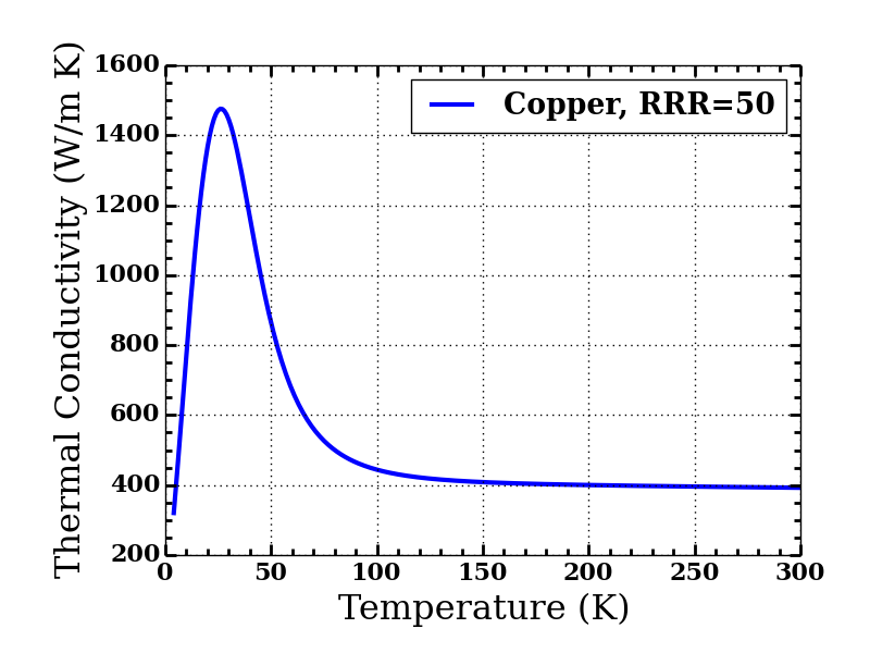
The thermal conductivity of copper as a function of temperature: We see a non-negligible change in thermal conductivity in the relevant temperature range for the HPF thermal copper strap; 77K to 180K. Data obtained from NIST’s cryogenic website – see here – assuming a Residual-Resistance Ratio (RRR) of 50 [RRR wiki – here].

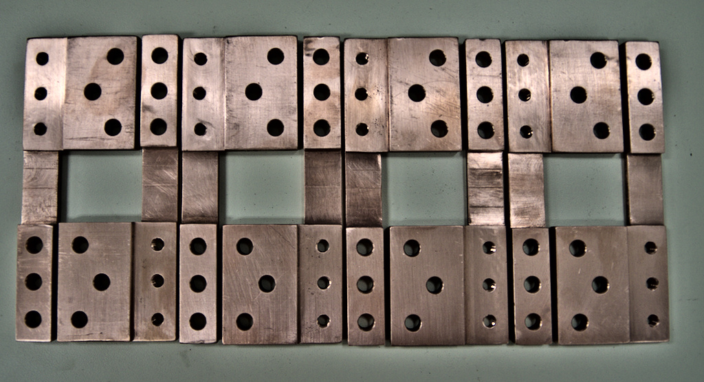
The images below show a few photos from the copper strap preparation; we will need 16 straps in total.

Milled and cut copper terminals: Cut and milled 110 multipurpose copper sheets, using a water jet, and a standard mill.

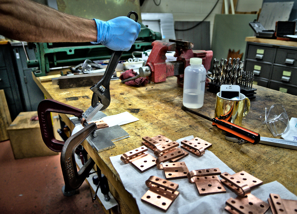
Bending Copper

A test Cu thermal strap

III. Heater Panels

Like mentioned above, the heater panels heat up the overcooled radiation shield to the 180K temperature goal. Each panel has 4 thermal resistors (150Ω each), which heat up in proportion to the electrical current going through them. As we now know the heat current from (I) the net incoming radiation, and (II) the copper straps, we can calculate the heat current needed from the heater panels to keep the system at equilibrium:

$H_{\mathrm{Heaters}}=H_{\mathrm{Cu}}-H_{\mathrm{rad}},$

which can be used to calculate the current needed per panel and per thermal resistor. The exact current running through per resistor is controlled by a thermal feedback control system which monitors any external temperature fluctuations at the observatory–we can’t control the weather! The system then compensates for these changes by controlling the amount of electrical current going through the resistors, warming them up as needed, keeping the instrument stable at 180K with the milli-Kelvin precision needed.

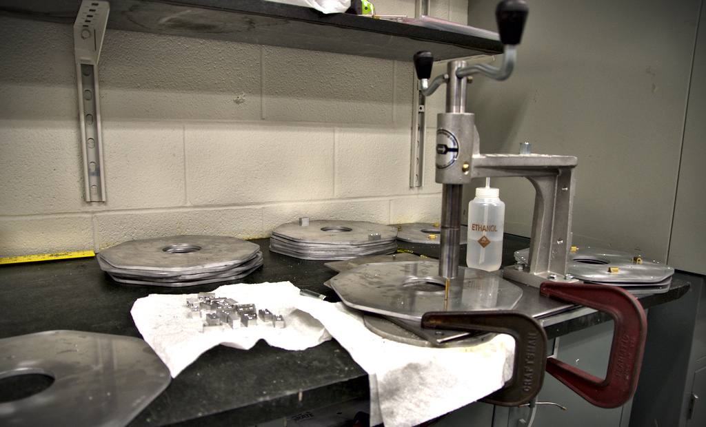
Tapping stage; each panel has 24 holes to be tapped; so that they can be bolted securely and with good contact to the radiation shield.

Thermal panel production: Tapping stage; each panel has 24 holes to be tapped; so that they can be bolted securely and with good contact to the radiation shield.

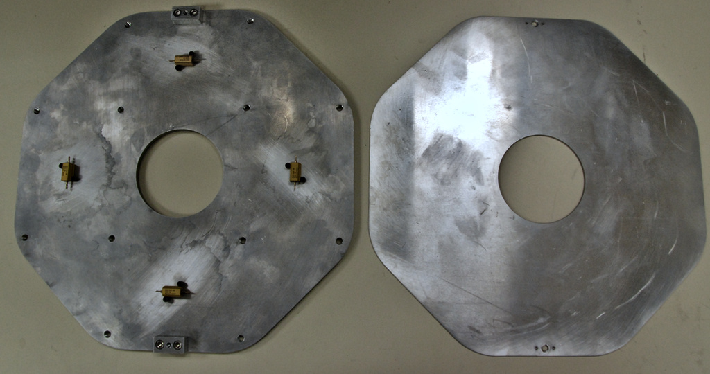
Aluminum Heater Panels:14 panels in total, each of which have 4 thermal resistors connected to the temperature feedback control system which is capable for keeping HPF stable at 180K.

Keeping it Cool