
The need for a good ruler
HPF is a high-precision spectrograph; it is designed to make very precise measurements of the wavelengths of stellar spectral features, so that the subtle Doppler shifts related to any orbiting exoplanets can be detected. We’ve discussed previously how this work requires a very reliable “ruler” to measure against; for HPF that is provided by a NIST-built laser frequency comb system.
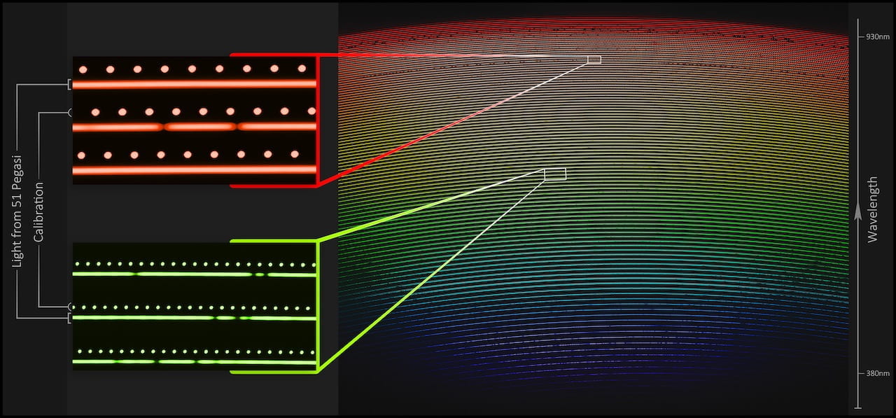
The stellar + calibration spectrum from NEID, a spectrograph similar to HPF. The regular lines from the laser frequency comb calibrator provide the “ruler” against which we can precisely measure stellar Doppler shifts.
The HPF laser frequency comb provides reliable, high-precision calibration for HPF. But, like most astronomical laser frequency comb systems, it is expensive and complicated. The innards of the HPF laser frequency comb are shown below to highlight its complexity – in many ways this system is more complicated than the HPF spectrograph itself!
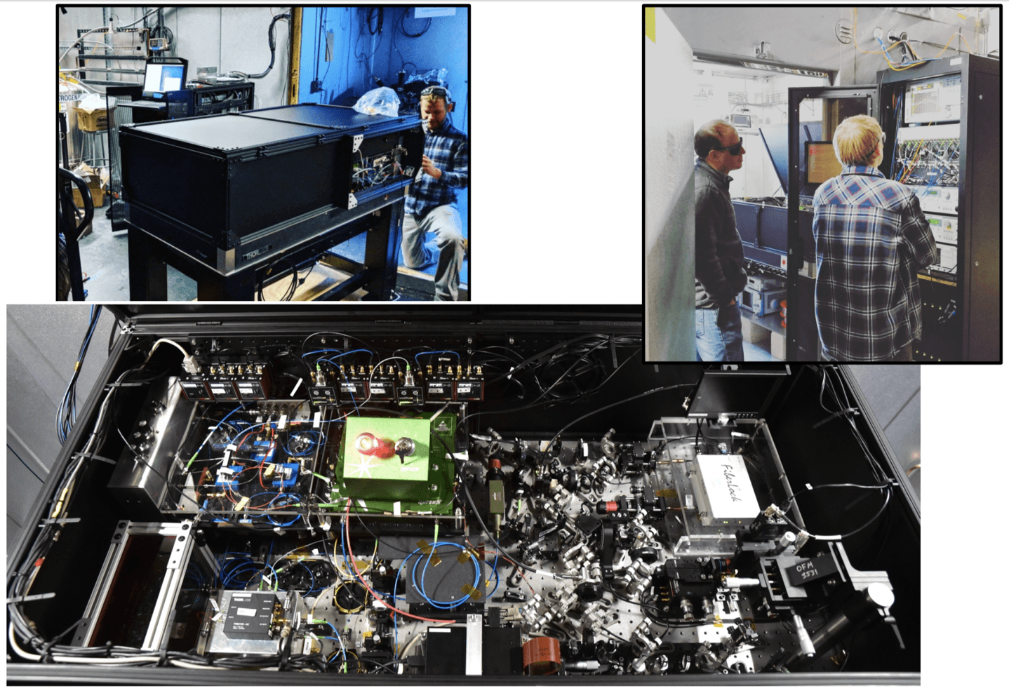
Photos from the installation of the HPF astro comb.
There therefore is a niche for a calibration source that provides high-quality calibration at a lower cost, and many Doppler spectrographs have converged on the use of Fabry-Pérot etalons for this purpose.
What is a Fabry-Pérot?
The ingenious idea behind a Fabry-Pérot etalon has been around for more than 100 years, and it is useful for many applications beyond the simple one discussed here. The idea is to place two partially-reflective mirrors next to each other and cause interference of incoming light, as shown in the figure below. An interesting property of this arrangement is that light waves between the mirrors can interfere with reflections of themselves (see the back-and-forth black arrows). This interference can be make the waves stronger (constructive) or weaker (destructive); it can only be constructive if the distance between the mirrors corresponds to a whole number of the light waves. This means that, if you illuminate the Fabry-Pérot etalon with a white light (all wavelengths), the spectrum inside of it looks like a comb (see below), where each bright line corresponds to a wavelength that “fits” inside. This is great for calibrating a Doppler spectrograph like HPF!
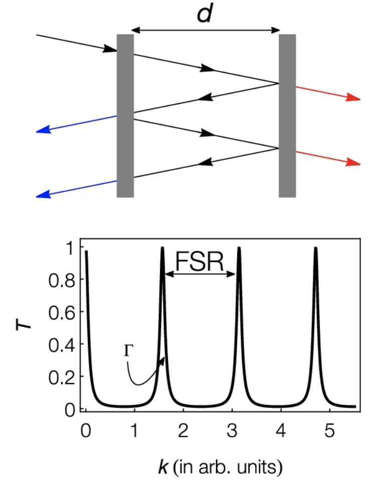
The top panel shows a schematic of a Fabry-Pérot etalon: incoming light of all wavelengths (from the left) passes through the partially reflective mirror and interferes with itself (black back-and-forth arrows). The output spectrum, shown in the bottom panel as a function of wavenumber (similar to wavelength), contains only the wavelengths that can “fit” between the mirrors.
Notice that which wavelengths show up in the output spectrum is directly related to the spacing between the mirrors. So, if the mirror spacing changes, the output spectrum will change too. Most groups (including us) that use Fabry-Pérot etalons want the spectrum to be very stable, so there is lots of careful engineering that goes into making the mirror separation as stable as possible. Ours, for example, is enclosed inside a temperature-stabilized vacuum chamber, much like HPF but on a smaller scale.
Even with this careful engineering, it is usually unavoidable that the mirror spacing slowly changes (a tiny bit) over the long term, and so the spectral lines should march slowly over time. So, the Fabry-Pérot etalon spectrum isn’t quite as good as the laser frequency comb, since the laser frequency comb lines stay at the exact same wavelength. But it is close!
A closer look
With HPF, we have an exciting opportunity to compare the spectrum of a Fabry-Pérot etalon (which can change over time) to the spectrum of a laser frequency comb (which stays put). This is exciting because even though Fabry-Pérot etalons are widely used, they are not commonly used for as wide a range of wavelengths as for HPF, so it is actually an open question how all the Fabry-Pérot lines (of which there are thousands!) will behave.
The result is a bit unexpected. Looking at a few examples of lines in different parts of the HPF spectrum, we see them marching like below: some lines appear to be moving blue-ward (their wavelengths are getting shorter) while some are moving red-ward (longer)!
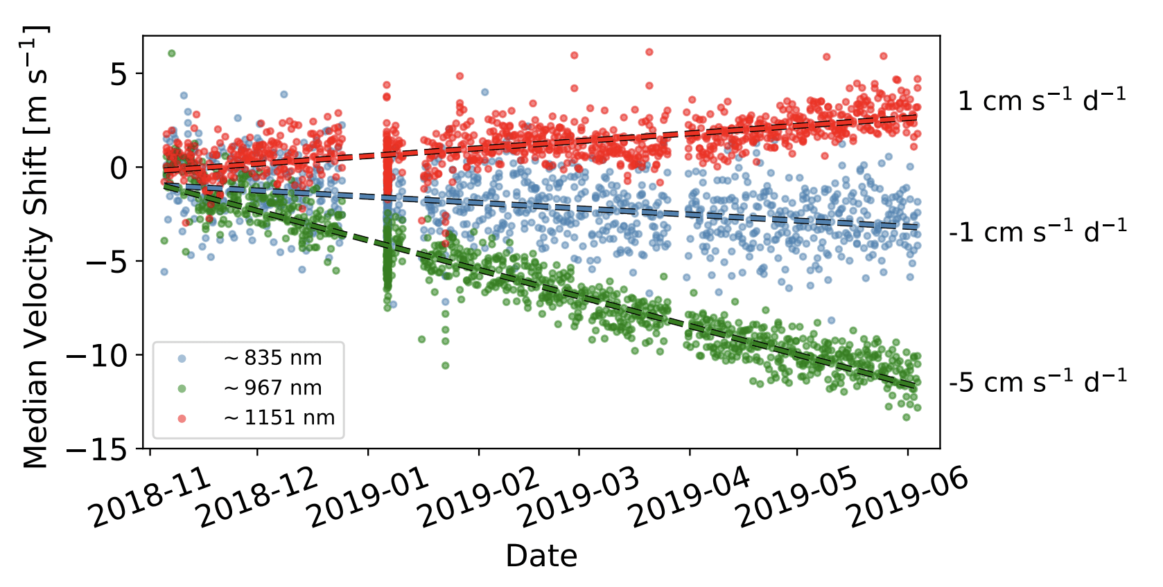
For three examples of Fabry-Pérot lines in different parts of the HPF spectrum, this is how they move over about 6 months. Some lines are moving towards smaller wavelengths (negative velocity shift), and some are moving towards larger wavelengths (positive velocity shift)!
This is interesting, because if the mirror separation were the only factor in play, the lines should at least agree on whether their wavelengths are getting shorter or longer. But this is decidedly not the case for our system, which means that there is something more complicated going on.
Zooming out a bit, we can look at all of the thousands of Fabry-Pérot lines in the HPF Fabry-Pérot spectrum, and see how they move over time. The plot below shows the slope of the line movement over time: each point on this plot shows how a single Fabry-Pérot line moves (on average) over many months. Points near 0 cm/s/d don’t move at all; points below 0 are steadily marching towards shorter wavelengths; points above 0 are marching towards longer wavelengths.
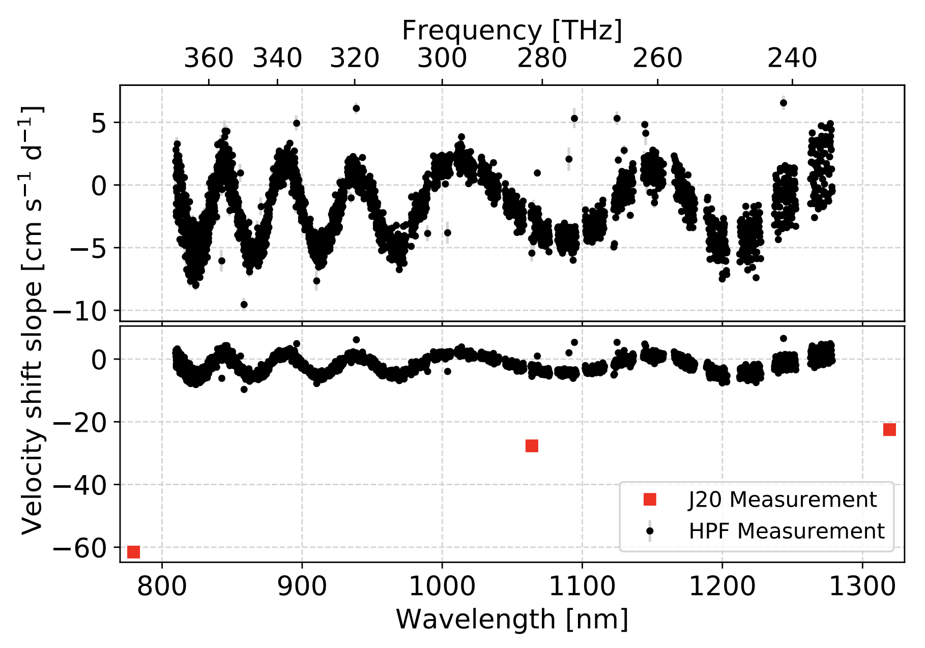
The average motion of the HPF Fabry-Pérot lines over the course of several months. Also shown (in the red points) are the measurements of the same quantity for this system with an entirely different method during pre-deployment testing, showing that it appears to have much less variability now.
This plot shows that the line movements are not just random: there is a clear pattern of variation across the spectrum. This oscillatory pattern could be related to small changes in the mirror itself, the way that light is shone into the Fabry-Pérot, or a host of other possibilities.
We also compared our new measurements to similar measurements we made several years ago before we deployed this Fabry-Pérot with HPF, and these are shown as the red points in the figure above (J20). Interestingly, the Fabry-Pérot lines seem to be moving much less than they were before – potentially indicating that the system has “settled down” to improved stability now that it is older.
Zooming out again, we found that even though the individual Fabry-Pérot lines are showing interesting behavior, they are not moving very much at all, and the overall spectrum is actually quite stable! One way of summarizing this is shown below: for different timescales what is the amount that the Fabry-Pérot spectrum has moved on average.

For different timescales, the average amount that the Fabry-Pérot varies. The monitoring dataset is chopped into different parts (Nov-June or Feb-June) to highlight that the system is actually more stable at some times.
This shows that, over days to weeks, the average velocity shift we measure with the Fabry-Pérot is reliable to <30 cm/s, which is great news for high-precision Doppler calibration!
Next steps
We are currently quite interested in the origin of the patterns we measured, and are working to test our various hypotheses and continue to monitor the behavior of the HPF Fabry-Pérot system. We are also attempting to measure the same properties of other systems, to see if this behavior is unique to our HPF system. Finally, we are working to fold in this new knowledge of our calibrator system to better calibrate HPF (and NEID) to achieve better precision for exoplanet detection.
Learn More
This work was recently accepted for publication in the Astronomical Journal, and a preprint of the paper can be found on arXiv. Our Fabry-Pérot was built by Light Machinery, and the system was assembled by Stable Laser Systems. Light Machinery has a super cool simulator that you can use to learn more about Fabry-Pérot etalons.
 RSS - Posts