The Year in Science: HPF Highlights 2014

It is important to remember that the team building HPF is not comprised of technicians dispassionately filling an order for a new machine, but instead includes many of the scientists who will eventually use the spectrograph for their own research.  We believe these collaborators’ enthusiasm for HPF’s science capabilities will be reflected in their contributions to the instrument, resulting in a spectrograph that is both better built and better used.

In addition to documenting the progress of the HPF build, we have taken the time on this blog to detail a lot of the exciting scientific research being produced by the team, in part because we find it especially gratifying to share our results with the public.  With that in mind, we are delighted to announce that two separate research projects led by HPF team members were selected to appear in Discover Magazine‘s top 100 science stories of 2014!

discover_crop

First, appearing at #59 is the exciting story of how Arpita Roy, Jason Wright, and Steinn Sigurdsson solved the 55-year-old mystery of why the far side of the Moon’s surface looks so different from the side we see from Earth.  The far side has a much thicker crust, and fewer of the dark “maria” like those we see in the face of the “man in the moon.”  According to Arpita and her collaborators, the difference can be explained by the increased temperatures on the Earth-facing side due to the heat radiating off the Earth, which was quite hot following the giant impact that formed the Moon.  You can get the full details of their work on Jason’s blog, or in the research paper.

Images of the near (left) and far (right) hemispheres of the Moon, from NASA's GRAIL mission.  Red/white colors indicate higher elevations, while blue/purple colors reflect lower elevation (Image courtesy NASA/GSFC/MIT/LOLA)

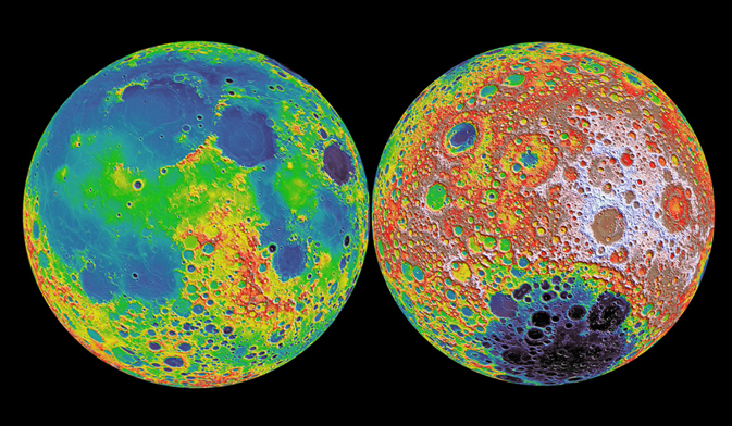
Images of the near (left) and far (right) hemispheres of the Moon, from NASA’s GRAIL mission. Red/white colors indicate higher elevations, while blue/purple colors reflect lower elevation (Image courtesy NASA/GSFC/MIT/LOLA).

Also sliding in as part of #100–which documents the year’s notable exoplanet arrivals and departures–is our work on stellar activity in the Gliese 581 exoplanet system.  This entry includes HPF team members Paul Robertson, Suvrath Mahadevan, Michael Endl, and Arpita Roy, thus marking Arpita’s second appearance in this year’s top 100 list!

As you can see, it has been quite a year in science for the HPF team.  Here’s to pushing back the frontiers  even more in 2015!

Posted in HPF Science | Comments Off on The Year in Science: HPF Highlights 2014

HPF Thermal Enclosure Setup at McDonald Observatory

Three members of the HPF team recently visited McDonald Observatory in Texas recently, with two goals in mind:

  1. Install the HPF thermal enclosure
  2. Setup a temperature monitoring system in the spectrograph room

DSC_1881

Installing the HPF Thermal Enclosure

The HPF spectrograph will sit in the Hobby-Eberly Telescope Spectrograph Room with light fed to it through a set of optical fibers from the telescope. It will sit in a thermal enclosure from Bally – yes one of those walk-in meat-locker coolers! It is perfect for our purposes, as the insulation box will act as a buffer to smooth out any short-time temperature variations (see confirmation of this in the graph below).

Below are a couple of pictures of the Hobby-Eberly Telescope Spectrograph Room before and after installation:

Before

Before installing the HPF thermal enclosure. You can see a) the HRS enclosure (white box on the left), b) the HPF calibration enclosure (silver box in the middle), c) some of the new uninstalled HPF enclosure panels, and d) the open area where the HPF enclosure will sit.

After

After installation: The HPF will sit inside this enclosure inside a clean room (not installed yet!) on the far side seen from this angle. A 6 foot sliding door – big enough for the HPF to get through – will cover up the remaining opening.

Moreover, you can see a short time-lapse video of the setup process right here:

Preliminary temperature monitoring system

During the last day we installed a temperature monitoring system (see figure below) devised by HPF team member Paul Robertson to measure temperatures at 6 places: high and low a) inside the Spectrograph Room, b) inside the Calibration Enclosure and c) inside the newly installed HPF enclosure. The placement of the sensors are summarized in the illustration below:

Temperature sensor Locations

Temperature sensor locations: Locations of the 6 PT-100 temperature sensors placed in 3 different locations high and low, summarized above.

Annotated photo of the temperature monitoring system, showing: a) An Uninterupted Power Supply (UPS), gracefully supplied by the Observatory, so if there is ever a power outtage we can still monitor the temperature! b) Raspberry Pi computer that logs the temperature from c) the LakeShore temperature monitor.

The temperature monitoring system: a) An Uninterrupted Power Supply (UPS), gracefully supplied by the Observatory, so if there is ever a power outage we can still monitor the temperature! b) Raspberry Pi computer that logs the temperature from c) the LakeShore temperature monitor which interfaces with the 6 PT-100 temperatures mentioned above.

 Nominally, the temperature in the Spectrograph Room is controlled to +-0.3°C, but we wanted to assess this independently, as any temperature changes will cause instrumental drifts, causing the overall radial-velocity precision to degrade. More specifically, our goals of installing the system were to monitor and gain insights into the following:

a) Low frequency temperature variations: These are long-baseline temperature changes, variations longer than a week. The temperature changes between the seasons are a good example. Do these drifts show up at all? If so, at what amplitudes? These questions are interesting as these drifts are the ones that HPF will notice, and where the active temperature control system will come in to compensate.

b) High frequency temperature variations: These are temperature variations around a day or less. Let’s say somebody opens the door to the outside and lets cool air come into the Spectrograph Room in the winter: we observe a temperature dip. In the summer: a temperature spike. Let’s face it: these variations are probably always going to be present. This is exactly why we have to install the thermal enclosure – to buffer these temperature fluctuations out. And, moreover, we want to install the system to get a concrete feel for how how effective these enclosures (the HPF and calibration enclosure) are at buffering out these high-frequency temperature variations.

Below we plot the first few days of temperature data obtained:

LakeShoreLogTotal

Temperature vs Time for the 6 temperature sensors from Nov 15 – Dec 2 (data for Nov 30 missing).

From the temperature plot above we can see the following:

1) The Calibration box (red curves), which is completely closed, shows that it very effectively buffers out high-frequency temperature changes in the Spectrograph Room (green curves).

2) The Calibration box (red curves) drifts with the longer-term temperature changes, as expected, but these same long-term temperature variations are higher than expected from the +/- 0.3°C control setpoint. This issue is currently under consideration. We will continue to monitor the temperatures carefully over the next months.


Posted in HPF Hardware, Project Development | Comments Off on HPF Thermal Enclosure Setup at McDonald Observatory

Fabrication of the Cryostat Vacuum Chamber

In order to preserve a cold, stable environment for the HPF optics, the entire instrument must be kept in a giant vacuum chamber, called a cryostat.  The cryostat must seal out the ambient atmosphere for years at a time, while simultaneously maintaining a rigid shape against the enormous forces of the external air pressure working to crush it like a soda can.  Needless to say, this is quite a challenge both to design and build!  Despite minor delays with regard to the machining of individual parts, the three primary assemblies for the cryostat shell are progressing very nicely, and are extremely close to completion.  Let’s take a closer look at the cryostat and its component parts.

The vacuum boundary is comprised of three assemblies. The box frame, the upper hood, and the lower hood.

IMG_2895

Here we see the box frame assembly. The ½” thick stainless steel perimeter seen on the top face of the upper box frame members will soon be machined to receive the large o-ring, responsible for keeping out as many air particles as possible.

When two components are welded together, they tend to distort relative to one another. Even with high capacity restraints, this fact is inevitable and unavoidable. The only thing one can do is to acknowledge that this distortion will take place, and plan accordingly. In this case, when the ½” plates are welded to the top of the box frame, and in fact even when the two sections of box members are welded together, they warp slightly. This is an issue, because in order to achieve uniform compression of the o-ring, this face must be as close to planar as possible. An o-ring is quite simply a rubber material, with a spherical cross section. When the o-ring is compressed between two plates, it fills any tiny imperfections in the surface of the plates. If done properly, an o-ring can be extremely good at keeping air out, allowing the HPF team to keep an extremely stable vacuum pressure within the cryostat. So in order to overcome the distortion induced by welding, and to achieve the flatness on this o-ring face that is required, the entire assembly you see in the photo above will be placed on a planar mill. The assembly will be restrained on the table, and the mill will then take several cutting passes, removing the upper layer of material, and leaving a surface that is flat to within 5 thousands of an inch (about the thickness of a dollar bill!). This same process will be repeated for both the upper and lower hoods, ensuring that any mating faces are as flat as possible.

The construction of the cryostat is truly an impressive process, and really must be seen to be appreciated.  Below, please enjoy some photos from our recent trip to the shop!

IMG_2873

Tack welds secure the o-ring plate during the welding process. The entire assembly is tack welded together, followed by stitch welds (connecting sets of tacks), or continuous welds where necessary.

IMG_2871

Here is a set of vacuum feed-through locations. A metal plate with an o-ring will bolt onto these faces, which you can see have been milled flat. By mounting hermetically sealed electrical connections on the metal plate, we are able to run wires and optical fibers into the instrument, as well as all necessary plumbing accessories.

DSC_0690

Checking the flatness of the top surface. The end caps were still not tack welded in place.

DSC_0711

Beautiful work


DSC_0689

Part of the HPF team discussing the welding progress on the upper hood. You can see the large clamps spaced around the perimeter, holding components in place during welding. Notice the aluminum foil wrapped around the clamps… always trying to keep things as clean as possible!

IMG_2896

This is the lower hood. It is nearly identical to the upper hood (seen in the background), except that it has 4 symmetrically placed circular penetrations. These will accommodate brackets designed to restrain the bench during shipment, keeping it from slamming into the cryostat body. Once the instrument is ready for operation, plates with gaskets will seal these 4 penetrations.

IMG_2870

Close-up of the end cap and support webs. When vacuum is drawn, these caps tend to deform into the cryostat volume. These three webs act as I-beams, keeping the ends from collapsing inwards. You can clearly see where the plate at the bottom of the photo was tack welded to the support beams, keeping it in place during the assembly process.


Posted in Uncategorized | Comments Off on Fabrication of the Cryostat Vacuum Chamber