
Introduction
Understanding how planets form and evolve is one of the fundamental topics of research in exoplanet science. How do planets and their atmospheres form? What are their atmospheres composed of, and how do they evolve with time?
The current understanding is that planets likely form in clouds of gas and dust, and planets similar in mass to Neptune or Jupiter are capable of retaining substantial gaseous atmospheres of hydrogen and helium. Throughout the evolution of a planetary system, the atmospheres of planets evolve as well, where substantial atmospheric mass loss is expected to occur in the first million years of their lives. During this time, the host star is active and releases considerable amounts of high energy radiation that is capable of eroding away exoplanetary atmospheres.
However, most planetary systems known orbit old stars—billions of years old—where the bulk of the atmospheric mass loss has already occurred, making it difficult to understand how the atmosphere evolved. With recent space-based missions such as the K2 mission and the TESS mission, a number of planets orbiting young stars have been detected. Enter the V1298 Tau planetary system: a promising young system for studies of atmospheric evaporation.

Figure 1: The young V1298 Tau system is composed of four planets known to transit its host star. The planets are expected to still be contracting and the high energy irradiation from the young star could be eroding significant amounts of their atmospheres away. Image credit: AIP/J. Fohlmeister.
V1298 Tau is a young K star (slightly cooler than the Sun) in the constellation of Taurus at a distance of 354 light years from Earth, recently discovered to host at least four transiting planets. The planets have orbital periods of 8.25, 12.4, 24.1, and >36 days. At an age of 23 million years, the system is one of the youngest planetary systems known to host multiple transiting planets. Being a young star, V1298 Tau is active and flares, bombarding the planets with high energy radiation. The planets are all observed to be large, and could still be contracting and cooling from their original formation condition. The young age of V1298 Tau, together with the expected extended atmospheres of the planets, makes the system exciting for studying evaporating atmospheres. Do the planets show signatures of ongoing atmospheric erosion? If so, how much?
These questions were the focus of a new paper accepted for publication in the Astronomical Journal led by graduate student Shreyas Vissapragada at Caltech and HPF team member Guðmundur Stefánsson. The paper is available on arXiv, and the key results are summarized below.
Measuring Evaporating Atmospheres in the Near-Infrared with the helium 1083-nanometer line
To probe for signatures of atmospheric erosion in the V1298 Tau system, we used the helium 1083-nanometer line. This line of helium is a relatively new way to measure the signatures of evaporating atmospheres. We have previously used HPF and the He 1083 nm line to detect the atmospheric evaporation of the M-dwarf planet GJ 3470b, which marked the first detection of He 1083 nm absorption in a planet orbiting an M dwarf. The line is produced by a short-lived transition of helium from an excited energy state to a lower non-excited state. Populating the excited state of helium in exoplanet atmospheres requires high energy X-ray/UV radiation, making planets orbiting young active stars particularly promising targets for such observations.
To probe if the V1298 Tau planets show signatures of evaporating atmospheres, we used two ways to investigate the He 1083 nm line: a) we used HPF on the 10m Hobby-Eberly Telescope, and b) we used specialized 1083 nm narrow-band filter observations on the 200″ Hale Telescope at Palomar Observatory.
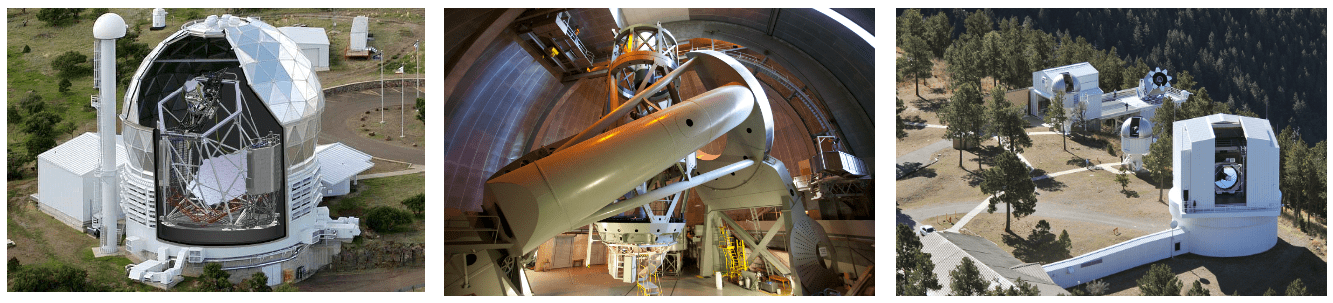
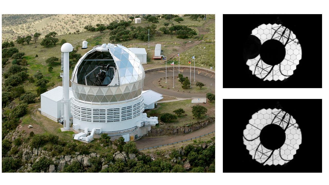
Figure 2: Telescopes used in this work: The 10m Hobby-Eberly Telescope at McDonald Observatory (left), the 200″ Hale Telescope at Palomar Observatory (middle), and the 3.5m Astrophysical Research Consortium 3.5m Telescope at Apache Point Observatory (bottom right). Figure credits: University of Texas at Austin, Palomar/Caltech, and Apache Point Observatory, respectively.
Transit Observations of V1298 Tau c with HPF and the ARC 3.5m Telescope
First, we used HPF’s coverage of the He 1083 nm line to look for evidence of helium absorption during the transit of the innermost planet V1298 c.
Figure 3a shows in-transit observations of V1298 Tau c using an Engineered Diffuser—nanofabricated pieces of optics enabling some of the highest precision photometric observations from the ground—on the 3.5m Telescope at Apache Point Observatory. We see a clear transit, along with a flare happening about an hour before the center of the transit. Simultaneously with these photometric observations we obtained HPF observations, where the timing of the HPF observations is denoted with the black triangles in Figure 3a. It is not often that you get spectroscopic observations in-transit and right after a flare!
The black spectra in Figure 3c show the combined spectroscopic observations from HPF during the in-transit observations, while the red, blue, and green spectra show HPF observations on different nights outside of transit. We see that the He 1083 nm line (three orange lines in Figure 3) is deepest during the transit: could that mean that we saw the helium absorption during the transit? It could be. However, we also see that the depth and shape of the line is highly variable, making it difficult to rule out the possibility that we are seeing intrinsic variations in the line from the star. Although non-conclusive, these observations give a direct constraint on the line behavior in-transit and outside of transit.
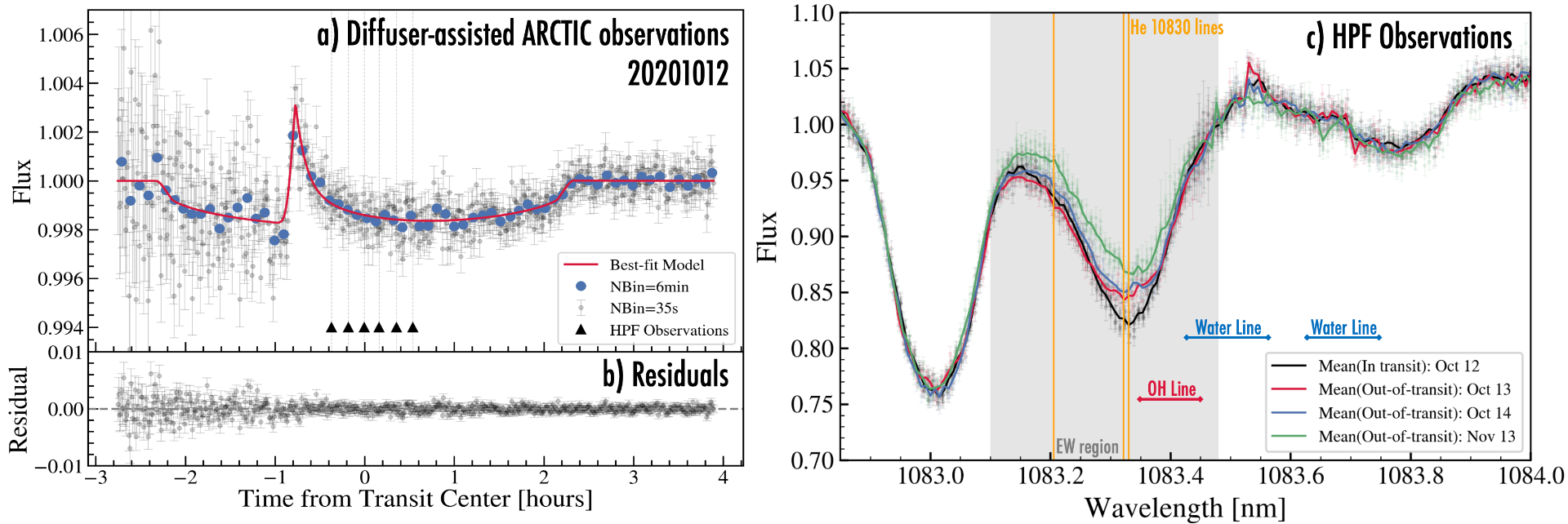
Figure 3: In-transit investigations of V1298 Tau c with HPF and ARCTIC on the 3.5m Telescope at Apache Point Observatory (APO). a) Transit from APO, showing a clear transit and a flare happening ~1 hour before the transit midpoint. b) Residuals from the transit and flare fit. c) HPF observations of the He 1083 nm line (denoted by the three vertical orange lines). In-transit observations are shown in black, while the red, blue and green spectra show out-of-transit comparison observations. We see that the line is the deepest during the in-transit observations. This could suggest atmospheric absorption, but we also see clear variability of the line in the other nights. As such, it is unclear if the variability is due to the planet or due to the activity of the star. Click image for full-size version.
Narrow-band diffuser-assisted observations of V1298 Tau c, d and b with the Palomar 200″ Telescope
Second, we used a specialized narrow-band filter centered on the He 1083 nm line developed by Shreyas Vissapragada for exactly these types of studies on the WIRC (Wide Field Infrared Camera) instrument on the 200″ Telescope at Palomar Observatory. You can read more on the specialized instrumental setup in a recent paper by Shreyas Vissapragada here.
Figure 4 shows the observations from the Palomar 200″ of V1298 Tau c, d and b. Planet c orbits closest to the host star, whereas planet b orbits furthest out (planet b was discovered first, hence the offset labeling). To see if we see signatures of excess absorption, we compare the transit depth we observe in the narrowband 1083 nm filter (shown in solid lines in Figure 4) to the known transit depths in broad-band filters (dashed lines). In Figure 4, we see that planets b and c show no clear evidence for increased transit depths. However, planet d shows a clear increased depth—a telltale signature of atmospheric absorption.
With planet d being the only planet showing a clear excess absorption, we discuss in the paper the possibility that planet d might be in a sweet spot for atmospheric erosion, whereas planets c and b might potentially be too close-in/far-out to create an absorption signal. Another possibility is that planet d is the lightest of the three planets, so it has the least amount of gravity to hold onto its atmosphere. We note that observations of planet d were performed on two different nights, so we urge additional observations that ideally cover a full transit in a single night to further confirm these observations and to look for variability in the transit depth from transit-to-transit.
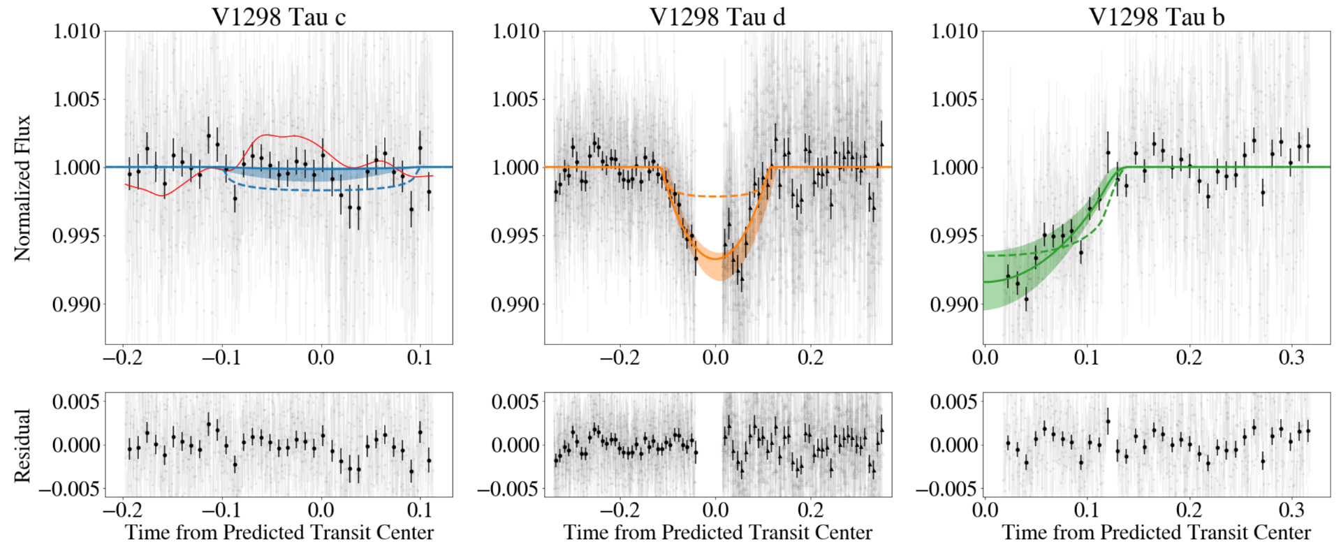
Figure 4: V1298 Tau observations of the transits of V1298 Tau c, d and b from the Palomar 200″ telescope using a purpose-built He 1083 nm narrow-band filter. Here we compare the expected transit depth in the He 1083 nm (solid lines) filter to previously known transit depth measurements (dashed lines). For planets c and b, we see transit depths that are consistent with previously measured transit depths. However, for planet d, we see evidence of a significantly larger transit depth.
With new young systems being discovered with increased frequency, we are excited to continue using HPF and these other instruments to study atmospheric evolution in different exoplanet systems to gain further insights into what drives atmospheric escape that ultimately sculpts the atmospheres we see for older more mature planets. For further information on this work, we invite you to take a look at the paper available on arXiv.


 RSS - Posts