A very stealthy alias: the impostor planet of Barnard’s star

Introduction

One of the signature targets of HPF’s search for nearby exoplanets is Barnard’s star, the second-closest star system to our own Solar system.  Barnard’s star made the news in late 2018, when the CARMENES team announced the discovery of a 3.3 Earth mass planet candidate orbiting Barnard’s star on a 233 day orbit. The star has long been a favorite among science fiction writers for setting their stories, so the discovery was met with great excitement by the public as well as the astronomical community. At the same time, the HPF team was observing this star as part of the instrument commissioning campaign, and we began analyzing the data in light of the new announcement. However, the more we looked, and the more data we collected, we did not see evidence for the planet signal. With the addition of nearly 120 new observations from HPF, and an analysis of archival RVs, we have concluded the proposed planet candidate is a false positive. The signal associated with the planet is in reality connected to the star’s 145 day rotation period.  This result is the subject of a new research paper led by HPF team member Jack Lubin; it will be published in the Astronomical Journal later this year, and you may access the preprint on arXiv for all of the technical details.

Background

Barnard proper motion

Barnard’s Star can be seen moving relative to background stars in this time-lapse image. Barnard’s Star has the highest on-sky velocity of any star. (Image courtesy Steve Quirk).

Since its discovery by namesake E.E. Barnard in 1916 from the University of California’s Lick Observatory, Barnard’s star has become one of the most well-studied of all the stars in the night sky. Astronomers in all subfields of stellar astrophysics have became fascinated by this star because it has the fastest movement across the sky of any star, relative to background stars.  Although, even if Barnard’s star were visible to the naked eye, you wouldn’t notice its motion by eye in your lifetime. We now know that it is the second nearest star system to our own Solar System at just over 5 light years, only beat out by the Alpha Centauri triple star system (thus Barnard’s star is the closest single star).

Barnard’s star has a colorful history when it comes to claims of exoplanets. In 1963, Peter van de Kamp at Swarthmore College published a paper on the star, claiming the first ever detection of an exoplanet. He used a method called astrometry, which measures if a star “wobbles” along the plane of the sky. If the star moves around in an ellipse in a characteristic and periodic motion, then we infer this motion is due to a planet gravitationally tugging on the star. Later that same year he published a follow up paper where he announced a second planet in the system and he refined both masses and orbits.

In 1973, John Hershey, also at Swarthmore College, revisited the same photometric plates as van de Kamp. He determined that all of the stars in the field of view near Barnard’s star were wobbling in the exact same fashion, implying an instrumental error. Hershey was able to point to various upgrades of the telescope that coincided with van de Kamp’s “wobbles”.  Also in 1973, George Gatewood from University of Pittsburgh and Heinrich Eichhorn at Wesleyan University published a paper finding no wobble in the star (and therefore no planets) using two different observatories.

Despite these papers showing the two signals van de Kamp published as planets were artifacts of his instrument rather than of astrophysical origin, van de Kamp never conceded. He even published two more papers in 1975 and 1982 refining the orbits and masses of his two planets. Sadly, Peter van de Kamp died in early 1995 believing he had discovered the first exoplanets, just months before the first confirmed exoplanet, 51 Pegasi b, was discovered by Michel Mayor and Didier Queloz, who both shared the 2019 Nobel Prize in Physics for their work. Later publications have definitively ruled out any planets in the Barnard’s star system with the masses and periods of those published by van de Kamp.

More Recent Planet-Hunting Efforts

Recently, an international collaboration led by the CARMENES Spectrometer Instrument team announced the discovery of a 3.3 Earth mass planet candidate orbiting Barnard’s star on a 233 day orbit. They used an expanded RV data set with 700+ observations taken over 23 years using 7 instruments. However, this purported planet’s orbital period is cause for concern. The stellar rotation period of Barnard’s star is around 145 days. How are these two numbers, 233 and 145, related to each other? They are one year aliases of each other.

Aliasing between a positive and a negative frequency

Examples of signal aliasing: two real signals (gold) are sampled at discrete points, shown by black dots. Using only the measurements at the sampling points, it is impossible to distinguish between the true signal and the higher-frequency alias shown in blue. Image credit: Andrew Jarvis, Wikimedia Commons

Aliasing is a phenomenon in signal processing whereby, due to incomplete sampling of a signal, we can be fooled into thinking a signal has a different period than it actually does . Aliasing is worsened when sampling a signal in unevenly spaced time intervals, as is the unavoidable case for all astronomical observations. Recall, in RV observations we are trying to measure the back and forth movement of the star by the shifting spectral lines. But other phenomena can also produce shifts in the lines, introducing additional signals into our data. Features on the surface of the star itself, such as starspots and other stellar activity, can induce shifts at timescales similar to the the rotation period or its harmonics.

These stellar activity induced signals can mimic a planetary signal, causing a false positive detection. Furthermore, unlike planet signals, stellar activity signals have a decaying nature, which makes aliasing worse. In exoplanet science, aliases most commonly occur with respect to astronomically significant time spans: 1 day, 1 lunar cycle, and 1 year.

New Data, New Conclusion

The HPF team began observing Barnard’s star 3 years ago as part of instrument commissioning. At the time we started, Barnard’s star was not known to host a planet. Soon after, the CARMENES team published their paper detailing the discovery of a planet candidate orbiting Barnard’s star. The HPF team continued observing the star, but as we compiled more and more data, we still saw no evidence for the planet. This prompted us to revisit the data upon which the discovery was based, and perform a joint analysis with our new HPF data.

First, we tested three different models of the system in an effort to discern which one described the data the best:

  1. A single planet with the same characteristics as claimed in the discovery paper, with no stellar activity
  2. The same planet, with an additional signal to describe the stellar activity of the star
  3. No planet, but with stellar activity

In accordance with Occam’s razor, if two models describe the data equally well, then the simpler model is preferred. When we compare our three models using only the data from the paper which claims the planet, we find the model which only accounts for stellar activity fits the data the best. This model is not the simplest model, but its extra complexity is justified by how much better it fits the data. When we repeat the experiment and include the newest HPF data, we find a similar result: our preferred model of the data is one which accounts for the stellar activity of the star, but without the proposed planet.

Barnard's star power spectra

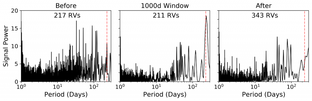
Power spectra of the radial velocities used to detect an exoplanet candidate orbiting Barnard’s star, separated into groups. The period of the purported planet is shown as a dashed red line. The signal appears strongly in a 1000-day region near the middle of the total time series, but not elsewhere.

Next, we reviewed the data year by year, finding that for three consecutive years near the middle of the data set, the signal associated with the 233 day planet was strongest. Meanwhile in other years, especially more recent years, the signal was very weak (even non-existent, like with the HPF data). This was highly concerning because while planet signals are persistent, activity signals are transient. The smoking gun is that in the same years that the signal at 233 days is strongest in the RV time series, there is also a strong signal at this same period in the spectral absorption features sensitive to stellar magnetic activity.

These tests combine to point us towards the conclusion that the proposed planet is instead an artifact of stellar activity manifesting at the one year alias of the rotation period. We are therefore compelled to return the planet of Barnard’s star to the shelf.

Importance and Impact

Barnard’s star is often considered to be the Doppler standard star for RV measurements of M dwarfs. This is due to its high apparent brightness, so even small telescopes can observe it, and its equatorial location, meaning telescopes in both the northern and southern hemispheres can access it. When commissioning new instruments, we often use Barnard’s star as a standard star, among others, because we believe we understand the star well enough that we can reasonably expect to know what the data should look like. Therefore if a new instrument returns different data, we are more likely to attribute the difference to the instrument, not the star. This helps the engineers and scientists refine the instrument and analysis methods.

But Barnard’s star has also been chosen as a Doppler standard because it is thought to be very quiet in nature, with little stellar activity. For decades this has proven true for instruments only capable of measuring signals of a few meters per second and larger. We are finding now, with the newest generation of spectrographs like HPF, that even Barnard’s star is in fact noisy below new, smaller thresholds.

Furthermore, this new paper represents one of the first studies to investigate how stellar activity from a long rotation period plays out over many seasons of data across multiple instruments. The rotation period of Barnard’s star is about 145 days, among the longest known rotation periods of any star! For example, our Sun rotates about once every 25 days, and many stars rotate faster than this. But this long rotation period is a significant portion of an entire observing season for Barnard’s star, which, depending on your latitude, is around 270 days. This long rotation period, coupled with the fact that starspots on M dwarfs can live through 10+ rotations of the star (whereas on our Sun, a starspot might live through only 3 rotations), means that spot-dominated activity on Barnard’s star could maintain high signal power for thousands of days, across multiple observing seasons. This is worrisome when it comes to signal sampling and aliasing. Future exoplanet studies where the host star is an M dwarf with a long rotation period will need to take extra caution when accounting for stellar activity.

In all, Barnard’s star has fascinated astronomers in all subfields for over 100 years, and the exoplanet subfield has a rich history with the star. It is vital to the astronomy community both for its astrophysical insights and for its use as a standard star among Doppler instruments. We may be ruling out this particular planet as a false positive, but the exoplanet community is not done with this star just yet. It is listed on the survey target lists for two new high-precision spectrographs, ESPRESSO and NEID, and the HPF team will continue to monitor Barnard’s star.

Posted in Exoplanet Science, HPF Science, Stellar Science | Comments Off on A very stealthy alias: the impostor planet of Barnard’s star

Wavelength-dependent behavior of the HPF Fabry-Pérot

The need for a good ruler

HPF is a high-precision spectrograph; it is designed to make very precise measurements of the wavelengths of stellar spectral features, so that the subtle Doppler shifts related to any orbiting exoplanets can be detected. We’ve discussed previously how this work requires a very reliable “ruler” to measure against; for HPF that is provided by a NIST-built laser frequency comb system.

LFC and Stellar spectra

The stellar + calibration spectrum from NEID, a spectrograph similar to HPF. The regular lines from the laser frequency comb calibrator provide the “ruler” against which we can precisely measure stellar Doppler shifts.

The HPF laser frequency comb provides reliable, high-precision calibration for HPF. But, like most astronomical laser frequency comb systems, it is expensive and complicated. The innards of the HPF laser frequency comb are shown below to highlight its complexity – in many ways this system is more complicated than the HPF spectrograph itself!

HPF Comb

Photos from the installation of the HPF astro comb.

There therefore is a niche for a calibration source that provides high-quality calibration at a lower cost, and many Doppler spectrographs have converged on the use of Fabry-Pérot etalons for this purpose.

What is a Fabry-Pérot?

The ingenious idea behind a Fabry-Pérot etalon has been around for more than 100 years, and it is useful for many applications beyond the simple one discussed here. The idea is to place two partially-reflective mirrors next to each other and cause interference of incoming light, as shown in the figure below. An interesting property of this arrangement is that light waves between the mirrors can interfere with reflections of themselves (see the back-and-forth black arrows). This interference can be make the waves stronger (constructive) or weaker (destructive); it can only be constructive if the distance between the mirrors corresponds to a whole number of the light waves. This means that, if you illuminate the Fabry-Pérot etalon with a white light (all wavelengths), the spectrum inside of it looks like a comb (see below), where each bright line corresponds to a wavelength that “fits” inside. This is great for calibrating a Doppler spectrograph like HPF!

Fabry Perot Schematic

The top panel shows a schematic of a Fabry-Pérot etalon: incoming light of all wavelengths (from the left) passes through the partially reflective mirror and interferes with itself (black back-and-forth arrows). The output spectrum, shown in the bottom panel as a function of wavenumber (similar to wavelength), contains only the wavelengths that can “fit” between the mirrors.

Notice that which wavelengths show up in the output spectrum is directly related to the spacing between the mirrors. So, if the mirror spacing changes, the output spectrum will change too. Most groups (including us) that use Fabry-Pérot etalons want the spectrum to be very stable, so there is lots of careful engineering that goes into making the mirror separation as stable as possible. Ours, for example, is enclosed inside a temperature-stabilized vacuum chamber, much like HPF but on a smaller scale.

Even with this careful engineering, it is usually unavoidable that the mirror spacing slowly changes (a tiny bit) over the long term, and so the spectral lines should march slowly over time. So, the Fabry-Pérot etalon spectrum isn’t quite as good as the laser frequency comb, since the laser frequency comb lines stay at the exact same wavelength. But it is close!

A closer look

With HPF, we have an exciting opportunity to compare the spectrum of a Fabry-Pérot etalon (which can change over time) to the spectrum of a laser frequency comb (which stays put). This is exciting because even though Fabry-Pérot etalons are widely used, they are not commonly used for as wide a range of wavelengths as for HPF, so it is actually an open question how all the Fabry-Pérot lines (of which there are thousands!) will behave.

The result is a bit unexpected. Looking at a few examples of lines in different parts of the HPF spectrum, we see them marching like below: some lines appear to be moving blue-ward (their wavelengths are getting shorter) while some are moving red-ward (longer)!

Mode slope examples

For three examples of Fabry-Pérot lines in different parts of the HPF spectrum, this is how they move over about 6 months. Some lines are moving towards smaller wavelengths (negative velocity shift), and some are moving towards larger wavelengths (positive velocity shift)!

This is interesting, because if the mirror separation were the only factor in play, the lines should at least agree on whether their wavelengths are getting shorter or longer. But this is decidedly not the case for our system, which means that there is something more complicated going on.

Zooming out a bit, we can look at all of the thousands of Fabry-Pérot lines in the HPF Fabry-Pérot spectrum, and see how they move over time. The plot below shows the slope of the line movement over time: each point on this plot shows how a single Fabry-Pérot line moves (on average) over many months. Points near 0 cm/s/d don’t move at all; points below 0 are steadily marching towards shorter wavelengths; points above 0 are marching towards longer wavelengths.

Mode Slopes

The average motion of the HPF Fabry-Pérot lines over the course of several months. Also shown (in the red points) are the measurements of the same quantity for this system with an entirely different method during pre-deployment testing, showing that it appears to have much less variability now.

This plot shows that the line movements are not just random: there is a clear pattern of variation across the spectrum. This oscillatory pattern could be related to small changes in the mirror itself, the way that light is shone into the Fabry-Pérot, or a host of other possibilities.

We also compared our new measurements to similar measurements we made several years ago before we deployed this Fabry-Pérot with HPF, and these are shown as the red points in the figure above (J20). Interestingly, the Fabry-Pérot lines seem to be moving much less than they were before – potentially indicating that the system has “settled down” to improved stability now that it is older.

Zooming out again, we found that even though the individual Fabry-Pérot lines are showing interesting behavior, they are not moving very much at all, and the overall spectrum is actually quite stable! One way of summarizing this is shown below: for different timescales what is the amount that the Fabry-Pérot spectrum has moved on average.

Binned deviation

For different timescales, the average amount that the Fabry-Pérot varies. The monitoring dataset is chopped into different parts (Nov-June or Feb-June) to highlight that the system is actually more stable at some times.

This shows that, over days to weeks, the average velocity shift we measure with the Fabry-Pérot is reliable to <30 cm/s, which is great news for high-precision Doppler calibration!

Next steps

We are currently quite interested in the origin of the patterns we measured, and are working to test our various hypotheses and continue to monitor the behavior of the HPF Fabry-Pérot system. We are also attempting to measure the same properties of other systems, to see if this behavior is unique to our HPF system. Finally, we are working to fold in this new knowledge of our calibrator system to better calibrate HPF (and NEID) to achieve better precision for exoplanet detection.

Learn More

This work was recently accepted for publication in the Astronomical Journal, and a preprint of the paper can be found on arXiv. Our Fabry-Pérot was built by Light Machinery, and the system was assembled by Stable Laser Systems. Light Machinery has a super cool simulator that you can use to learn more about Fabry-Pérot etalons.

Posted in HPF Hardware | Comments Off on Wavelength-dependent behavior of the HPF Fabry-Pérot

The Mysterious Blue Ring Nebula Uncovered

The Blue Ring Nebula is a rare and peculiar object composed of gas expanding from a central star, and is the subject of the most recent paper involving data from HPF. The Blue Ring Nebula (Figure 1) was originally discovered in data from NASA’s GALEX spacecraft, a spacecraft which scanned the sky at ultraviolet wavelengths. In its survey of the night sky, GALEX uncovered an intriguing nebula of hydrogen gas rapidly expanding from a star at its center. What are the properties of the star? How was the expanding material ejected? Data from HPF was key to help answering these questions. Our findings are reported in the latest issue of Nature.

Figure 1: The Blue Ring Nebula is composed of expanding hydrogen gas (blue nebula, and red filaments) from a central star (yellow star in the center). Data from HPF at the 10-meter Hobby-Eberly Telescope at McDonald Observatory helped uncover the properties of this peculiar and rare object. Image credit: NASA/JPL-Caltech/M. Seibert (Carnegie Institution for Science)/K. Hoadley (Caltech)/GALEX Team.

A hypothesis: A Result of a Binary Star Merger?

Most stars in the Galaxy are binary stars, and thus have an orbiting companion star. As stars age and evolve, their layers expand. Very massive stars end their lives in an explosive supernova, and can leave behind a neutron star or a black hole. In some binary systems, the expanding star can engulf the companion star, causing the binary companion to spiral in and the two stars to merge. Some such binary mergers have been observed before. However, in the hustle and bustle of the inward-spiraling death dance, which ejects and throws around dust and gas, the resulting remnant star often becomes completely enshrouded by opaque material, making the properties of the remnant star difficult to probe, and the whole merging process difficult to understand.

The Blue Ring Nebula shows many of the indications of such stellar mergers: ejected material expanding at rapid velocities from a central star, with accompanying signatures of shockwaves. There is one key difference from all the other objects: we can clearly see the central star, offering a pristine window into its properties. Could it be a stellar merger? Spectroscopic data from 10 meter-class telescopes helped uncover the mystery.

High Resolution Spectroscopy from 10 meter-class Telescopes

To better understand the properties of the Blue Ring Nebula, the team—led by Dr. Keri Hoadley at Caltech—obtained both precision radial velocities (RVs) from the HIRES spectrograph on one of the two 10-meter Keck Telescopes in the optical and HPF on the 10-meter Hobby-Eberly Telescope (HET) at McDonald Observatory in the near infrared. Figure 2 shows RVs from both HPF and Keck. The initial optical RVs potentially suggested a periodic variability at ~13.75 days, which could have been suggestive that the central star still had an orbiting companion. However, further scrutiny into the shapes of the stellar spectral lines, along with additional RVs from HPF in the near-infrared—which are less sensitive to certain types of stellar activity—revealed a highly active star. Clear correlations are seen with the RV variability with activity indicators, suggesting the RV variability is due to activity on the star rather than an orbiting companion. In particular, the HPF Differential Line-Width Indicator (dLW)—a measure of how the average widths of the lines in the HPF spectra are changing—shows a clear variability (Figure 2c), suggesting that the RV variability being measured is due to the shapes of the lines changing. This is also seen in data from the optical spectra (Figure 2b).

Blue Ring Nebula RVs

Figure 2: Precision RVs and activity indicators from Keck/HIRES (upper panels) and HET/HPF (lower panels). Initial RVs from Keck/HIRES (a) potentially suggested that there might be a low-mass companion orbiting the central star. However, further scrutiny into activity indicators (panels b, c, and d) along with data from HPF (panel c), suggested that the RV variations likely originated from activity from the star instead of an orbiting companion. These data rule out the possibility that there is a massive object orbiting the central star, yielding critical insights into the properties of the final remnant star at the center. Figure adapted from Hoadley et al. 2020.

Together with the high resolution spectra, coupled with other data from a number of space and ground-based observatories, along with detailed theoretical modeling, the Blue Ring Nebula is consistent with the picture of a stellar merger, where the primary star likely engulfed a low-mass star only a few thousand years ago. As the Blue Ring Nebula is the only binary merger known with a clear view of the central star, it yields particularly variable insights into the properties of such stellar remnants, and how the merging process unfolded. Although the Blue Ring Nebula is a rare object, it will be interesting to see if more such objects are found with future observations from space observatories scanning the sky. This would help yield further insights into how tight stellar binaries meet their demise.

Posted in HPF Science, Stellar Science | Tagged , , , | Comments Off on The Mysterious Blue Ring Nebula Uncovered