G 9-40b: HPF’s first planet validation

HPF has validated its first planet called G 9-40b, a sub-Neptune sized planet (2 Earth radii) orbiting a nearby low mass M-dwarf star with an orbital period of 6 days. The paper has been published in the Astronomical Journal and is available freely on the arXiv preprint server here.

It takes a Village to Validate a Planet

What does it take to say that a planet candidate is a bone-fide planet? Even for promising planet candidates around nearby stars, it takes a number of follow-up observations to say that a planet candidate is really a planet, and not something else, such as an eclipsing binary star system or other astrophysical false positives that can imitate planet transits.

G 9-40 was originally presented to have a candidate transiting planet in a paper by Yu et al. 2018 using photometric data from the K2 mission. After a closer look at this candidate planet, we saw it looked interesting for many reasons.

First, at a distance of only ~90 light years, G 9-40b is among the 20 closest transiting planetary systems known (see Figure 1), and is currently the second closest transiting planets discovered by the K2 mission to date. Second, the host star is a nearby bright M-dwarf star—but being bright makes it easier for us both to get a good radial velocity precision on this target with HPF, and to observe additional transits of it from the ground at high precision. Further, the brightness of the host star along with the large transit depth of the planet (~0.35%, see Figure 2) makes G 9-40b one of the most favorable sub-Neptune-sized planets orbiting an M-dwarf for transmission spectroscopy with the James Webb Space Telescope (JWST) in the future—more on that below.

Figure 1: Planet radius as a function of the distance of the planet system from Earth in parsecs (1 parsec is about 3.2 light years). G 9-40b (highlighted in the bright red) is among the closest transiting systems known to date. Red points show planets around low mass stars (M-dwarfs) and blue points show planets orbiting more massive hotter stars. Figure 12 from the paper.

Given these reasons, we decided to conduct more observations of this planet candidate and characterize it better to decide if this was a planet or not. To do so we used Adaptive Optics (AO) imaging observations, further precision transit follow-up observations from the ground, and precision radial velocities with HPF. Lets dive into each of these observations below.

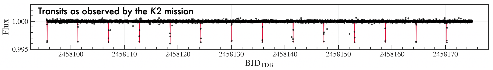
Figure 2: Transits observed in the light curve of G 9-40 from the K2 mission. The transits are deep, making it a compelling candidate target for transmission spectroscopy in the future with the James Webb Space Telescope. Figure 7c from the paper.

Adaptive Optics Imaging

To check if G 9-40 is blended with another star—which could confuse us on which star is the true source of the transit, or indicate that the system would be an eclipsing binary system rather than a true planet—we used high contrast adaptive optics imaging observations from the ShaneAO system at Lick Observatory. These adaptive optics observations are often conducted by shooting a high power laser into the air (Figure 3) to generate a so-called laser guide star. This laser guide star is then used to correct for the distortion in the atmosphere by rapidly changing the shape of an ‘adaptive’ mirror in the optical system, allowing us to obtain extremely high contrast images of the star. From these observations we see no evidence of blending or other stellar companions nearby the star G 9-40, further suggesting that G 9-40 is the true source of the transits we see from K2 and in our ground-based data (see next section).

Figure 3: Adaptive optics image (left inset) and resulting contrast curve as observed with the ShaneAO Adaptive Optics (AO) System on the 3m Shane Telescope at Lick Observatory (right). The contrast curve on the left shows the brightness of the inset image (in the near-infrared K-band) as a function of the distance from the center of the star. We see no evidence of a background star in the image that could dilute and/or be the source of the transits we see in the K2 and/or ground-based data. Left: Figure 1 from the paper. Right image credit: Laurie Hatch.

Ground-based Transit Photometry using Engineered Diffusers

To constrain the planet parameters and further update the orbital ephemeris of the system, we used high-precision diffuser-assisted photometry using the ARCTIC imager on the 3.5m Telescope at Apache Point Observatory. We observed the transit using a custom-built narrow-band filter made by Semrock / AVR Optics  that operates in a band with little-to-no water absorption. We often call this filter the ‘cloud-killer’. If you are interested, you can actually buy a very similar filter from Semrock off-the-shelf here!

The plot below shows our ground-based transit, which agrees well with the transits observed by K2 further suggesting that our planet candidate is indeed a planet. Further, these observations allow us to pinpoint the timing of the transit extremely well, allowing us to predict midpoints at the start of the JWST era (~2021-2023) with less than 2minutes of error. Such small errors are important to enable easy scheduling for in-transit spectroscopic follow-up in the future.

Figure 4: Transit observations of G 9-40b. Left: Ground-based transit measurements—showing the flux of the star as a function of time, showing a clear transit dip—obtained using the ARCTIC imager and the Engineered Diffuser on the 3.5m Telescope at Apache Point Observatory (right). These observations allow us to further characterize key parameters of the planet, including its period and its radius. Image credit: Figure 7e from the paper (left), Gudmundur Stefansson (right).

But what is the diffuser-assisted photometry? Excellent question. This means that we used recent technology called Engineered Diffusers—developed by RPC Photonics—to help conduct the observations. Engineered Diffusers are nano-fabricated devices that you can easily place in a telescope beam-path to mold the focal plane image of a star to a stabilized top-hat shape (Figure 5). In doing so allows you to keep the image of the star stable throughout the night, minimizing photometric errors due to the atmosphere. Further, in spreading out the light over many pixels opens up the possibility to observe bright targets on large telescopes—especially useful in observing G 9-40—with the 3.5m Telescope at Apache Point Observatory. If you are interested in reading more about Engineered Diffusers for astronomy you can read more about them in a past press release here or here, or in our previous paper here.

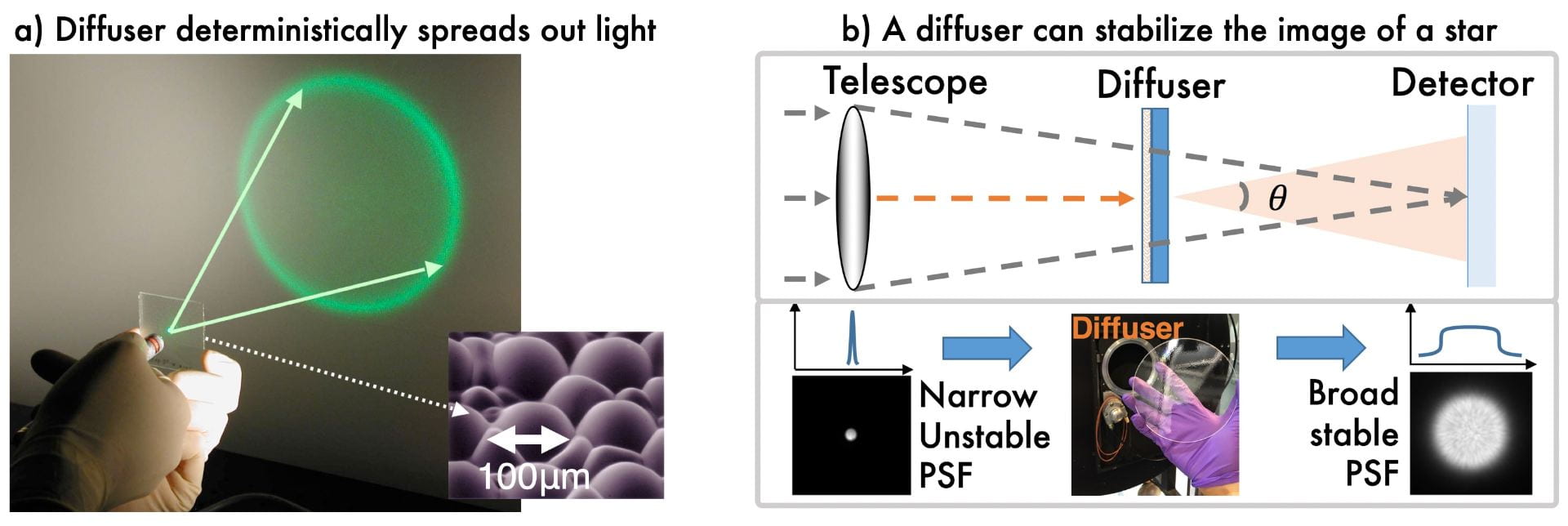
Figure 5: An Engineered Diffuser is capable of molding the image of a star into a broad and stable top-hat shape. b) We used an Engineered Diffuser in the telescope beam path of the 3.5m Telescope at Apache Point Observatory to stabilize the image of the star and allow us to obtain extremely high photometric precisions allowing us to precisely characterize the parameters of G 9-40b. Image credit: RPC Photonics (left), Gudmundur Stefansson (right).

Precision Radial Velocities from HPF

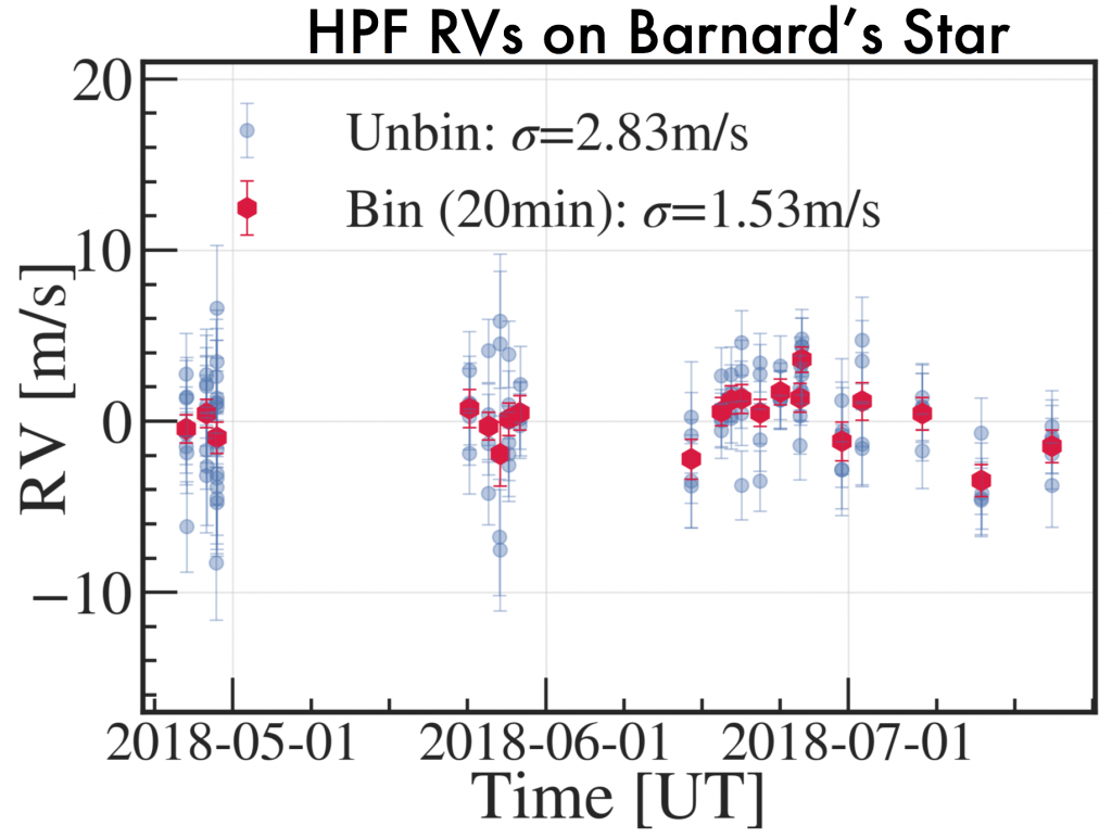
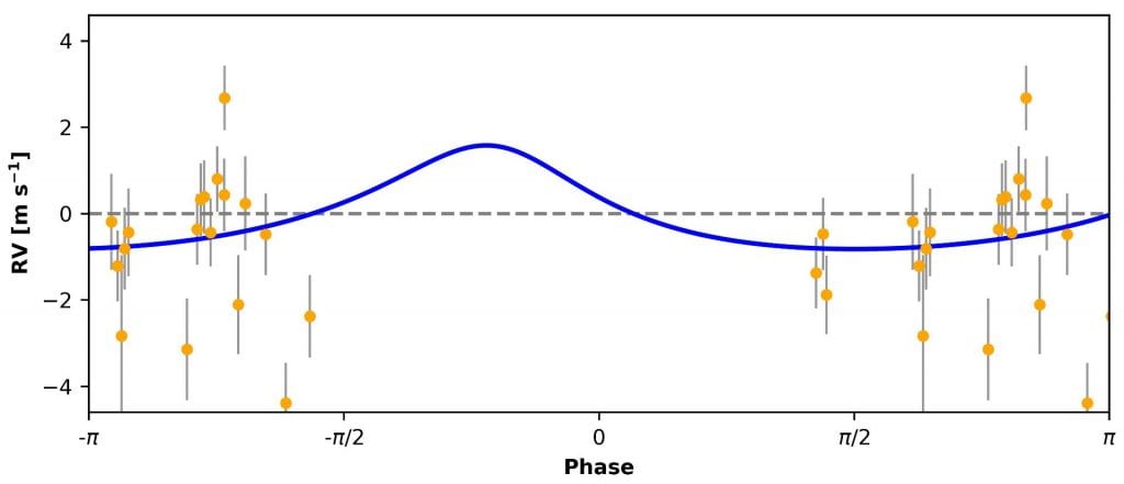
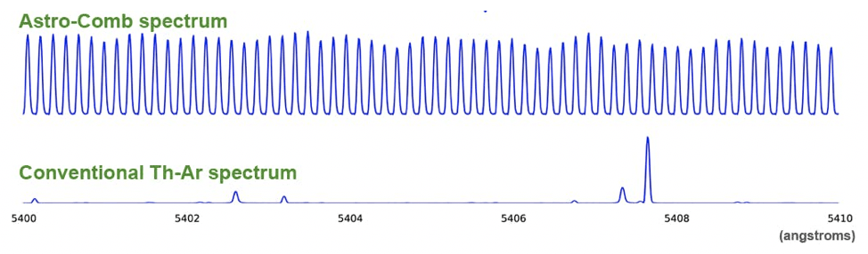
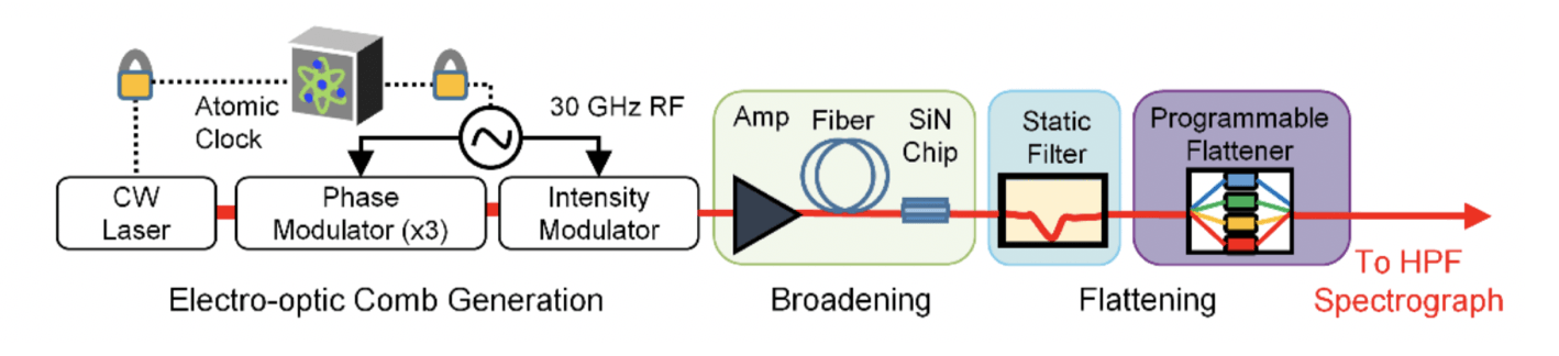
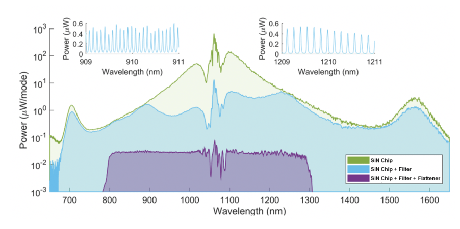
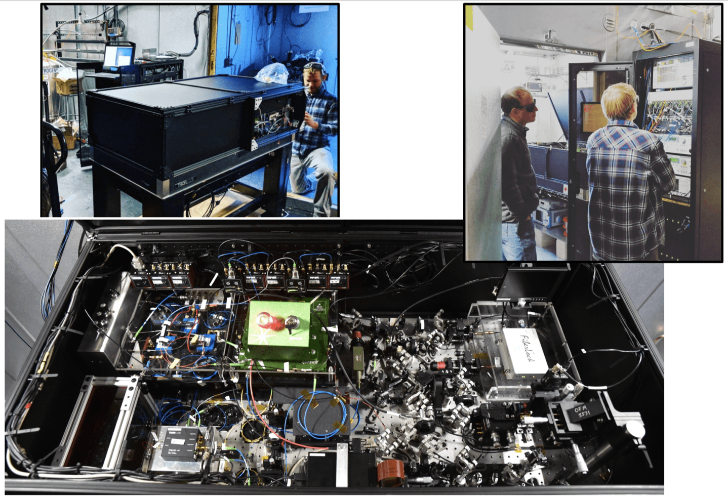
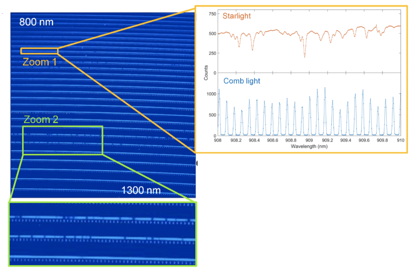
Last but not least, this paper includes some of the first precision near-infrared (NIR) radial velocities (RVs) from the Habitable-zone Planet Finder. In a previous paper led by AJ Metcalf, we showed that HPF is capable of 1.5m/s RV precision in the NIR (see blog post here), enabled by the precise near-infrared HPF Laser Frequency Comb (LFC) also discussed in detail in our previous blog post here. Using precision NIR RVs from HPF enabled by the HPF LFC, we placed an upper limit on the mass of G 9-40b of 12 MEarth. We hope to obtain a robust mass measurement with future RV measurements with HPF in the future. In doing so will allow us to constrain the composition of the planet, and to inform future atmospheric follow-up efforts with JWST.

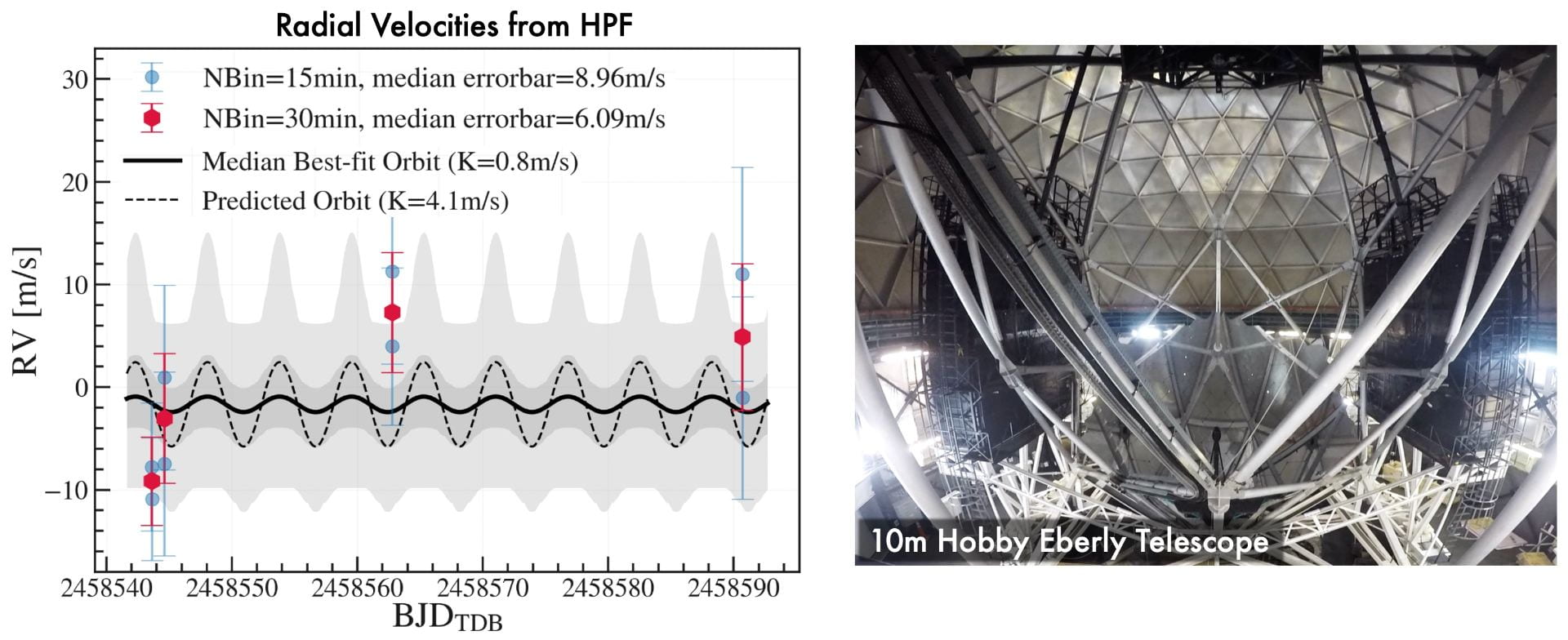
Figure 6: Precise radial velocities from HPF (left) on the 10m Hobby-Eberly Telescope (right) allowed us to place an upper limit on the mass of the planet of 12 Earth masses. We hope to get a further precise mass constraint by continuing to observe G 9-40 in the future. Image credit: Figure 11a from the paper (left), Gudmundur Stefansson (right).

Posted in Uncategorized | Comments Off on G 9-40b: HPF’s first planet validation

HPF Commissioning: A New Standard in the Near Infrared

We’ve been quiet…

Our last post, made about a year ago, shared our excitement at having delivered HPF to its permanent home on HET, and recording the instrument’s first data.  Since then, we have been busy doing the hard work of “commissioning” the instrument.  For an astronomical instrument, commissioning refers to a period of performance verification and fine-tuning that occurs once the instrument arrives at the telescope.  Certain tests and adjustments can only be done in conjunction with the telescope, so some patience is required as the instrument team makes improvements before real science can begin.

We are happy to report that HPF has now been released to the HET community for full science operations!  We have also collected enough data that we can start to evaluate the measurement precision of the spectrograph, and determine whether our on-sky performance matches our original project goals.  Here, we will show you some of that data, and explain why we are confident that HPF will break new ground in the study of the nearest exoplanet systems.  Technical details of this work can be found in an upcoming edition of Optica.

Barnard’s Star: the M Dwarf Standard

While the ultimate goal of any Doppler spectrograph is to find lots of exoplanets, boring is better during the commissioning phase.  The only way to test the stability and precision of your end-to-end measurement system–from the telescope, through the fiber optics, and ultimately the optics and detector of the spectrograph–is to make repeated measurements of a star with little or no variability.  That way, any variability seen in the measurements must be caused by the instrument, rather than the star itself.  In other words, the less variability we measure in observations of our stable “standard star,” the better the instrument is performing.

For the M dwarf stars HPF is designed to target, the best standard star is also one of the most famous stars in the sky.  Barnard’s star–named for the American astronomer E. E. Barnard–is the second-closest star system to the Sun (after the alpha Centauri triple system).  It is a little more than 14 percent as massive as the Sun, which is typical of the stars HPF will survey for exoplanets.

Barnard’s star can be seen moving relative to background stars in this time-lapse image. Barnard’s star has the highest on-sky velocity of any star. (Image courtesy Steve Quirk).

Barnard’s star is extremely old–possibly as old as the Milky Way Galaxy itself.  As such, it is rotating extremely slowly, and exhibits little of the stellar activity that causes radial velocity variability in other stars.  That low variability makes it an excellent commissioning standard for HPF.  Furthermore, its location near the celestial equator means it has been observed by telescopes in both the Northern and Southern Hemispheres, so we can compare our results to those of other spectrographs.

 The Observations

The Hobby-Eberly Telescope is queue scheduled, meaning resident astronomers record data for multiple users over the course of a single night.  This method of scheduling is ideal for repeated observations of a single star over time.  From February through July of 2018, HPF recorded the spectrum of Barnard’s star on every night possible.

Our HPF observations kicked into high gear in May, when the Laser Frequency Comb (LFC) from our team members at NIST and CU was fully operational at the HET.  The LFC is based on Nobel-prize-winning technology, and uses carefully modulated lasers and optics to create a perfectly uniform array of laser lines that can be used to provide an ultra-stable wavelength reference against which HPF measures Doppler shifts in a star’s spectrum.  We discuss the LFC in more detail in a companion post.

By the time we shut down HPF for some post-commissioning maintenance, we had made 21 high-quality measurements of Barnard’s star using HPF with the LFC.  These observations span 86 days, which is enough to quantify the baseline stability of the HPF system.  Let’s take a look at the results:

The Results

We would be remiss if we did not emphasize that working all of the kinks out of an ultra-precise Doppler spectrograph is a years-long process, and we are far from done making improvements to the instrument and our analysis techniques.  With that said, our early observations of Barnard’s star are extremely promising!

HPF radial velocities of Barnard’s star. Blue points represent individual spectra, while red points are the average of measurements made within a 20-minute series. The 1.5 meter per second precision is the best ever achieved in the near infrared!

Our current data series on Barnard’s star show a stability of around 1.5 meters per second, which is the best ever demonstrated on an infrared instrument.  For comparison, the most stable measurements of Barnard’s star ever reported come from the HARPS spectrograph, and they check in at around 1.2 meters per second.  Until now, HARPS has been the industry standard in ultra-precise Doppler spectroscopy, so for HPF–with its newer and more complicated infrared technology– to nearly match HARPS so soon after going on sky is a major accomplishment!

Long-time readers of this blog may recall that our goal measurement precision is 1 meter per second, while our current precision appears to be around 1.5 meters per second.  What noise sources might be remaining?  It is probably a combination of stellar activity, contamination from Earth’s atmosphere, small exoplanets, and some yet-to-be identified instrumental systematics.  We are continuing to check everything in an effort to squeeze every last drop of precision out of HPF.

A Planet Around Barnard’s Star?

Just after we finished our commissioning observations on Barnard’s star, the Red Dots team announced they had discovered a candidate exoplanet orbiting Barnard’s star.  The proposed planet, Barnard b, is around 3 times the mass of the Earth and takes 233 days to complete an orbit, so its Doppler signal is quite small.  Nevertheless, HPF’s precision is good enough to at least see some trace of this planet, so what gives?

As it turns out, cosmic coincidence prevents us from having much information on Barnard b at this point.  The orbit of the proposed planet is eccentric, which means the Doppler signal is more pronounced at some phases of its orbit than others.  Through nothing but luck, our HPF-LFC observations completely missed the most dynamic section of the Barnard b phase curve.

The orbital model of Barnard b (blue), with HPF measurements (gold) folded to the orbital phase. Our measurements have not yet covered the maximum of the eccentric orbit.

Thus, while our HPF measurements do not rule out the proposed planet, they cannot yet confirm it, either.  This is just one of many examples of how exoplanet detection is a data-intensive process!

Conclusion

HPF’s first year on sky is in the books, and things are looking quite promising!  We are already setting new records for Doppler precision in the near-infrared, and continue to push towards even better stability.

Now, the fun part begins.  HPF science operations officially started on December 1, 2018.  Whereas Barnard’s star is one of the most familiar, well-studied stars in the sky, we will now expand our operations to examine stars about which relatively little is known.  As always, we will share any exciting new results with you here.

We will continue to observe Barnard’s star, both to validate our long-term instrumental performance, and to learn more about any planets that may orbit this ancient star.  It is as quiet as stars come, but it may still be harboring some exciting secrets.

Posted in Exoplanet Science, HPF Hardware, HPF Science, Project Development | Comments Off on HPF Commissioning: A New Standard in the Near Infrared

The HPF Astro-Comb

After beginning operations earlier this year, HPF continues to patiently watch for the subtle Doppler shifting of stellar spectra that hints at the back-and-forth tug of orbiting exoplanets. As described in previous blog posts, HPF records spectra on a detector array (similarly to how a digital camera records an image), and the shifts we seek amount to microscopic motions of the spectra back and forth by just a few nanometers!

To be able to detect this shifting, we have engineered HPF to be very stable – the optics and detector are built from special materials and mounted carefully so that they don’t cause any shifts of the spectra that could be misinterpreted as Doppler shifts. We’ve carefully thought about all the potential causes of “false” Doppler shifts, from slight thermal changes moving the diffraction grating to systematically weird ways that the light can be launched from the fiber into the spectrograph.

However, this precision engineering doesn’t eliminate the “false” Doppler shifts, which are often referred to as “drifts” of the spectrograph. Even with a perfectly still, unmoving stellar spectrum shining into the telescope, we would still observe the spectrum moving in position by a few nanometers on the detector. These drifts may be attributable to any number of physical causes, from mechanical relaxation of optical components to slight differences in the weight distribution of the optical bench when we fill up HPF with liquid nitrogen coolant every day.

No matter the cause, these drifts must be corrected if we hope to detect the true ~1 meter per second signals from habitable zone planets orbiting M dwarfs. We go about correcting the measurements by measuring the spectra of two sources at once: one being the star of interest, and the other being a calibration source that is known to stay as still as possible. Any measured drifts of the calibration spectrum should be entirely due to “false” Doppler shifts. We can then subtract these from the measured shifts of the stellar spectrum, which contains both the “true” Doppler shift of the stellar spectrum as well as the drift. This isolates the “true” Doppler shift of the star (or more precisely, the relative motion between the star and the Earth).

What types of spectra can we use for this calibration?

An ideal calibration spectrum should have spectral lines throughout the region we are measuring, and those lines should be as stable as possible. The lines should also be roughly uniform in brightness, because we don’t want the detector to be blinded by one spectral line that is much brighter than the others.

Historically, the main option available for such calibration has been atomic emission lamps. These lamps are filled with certain well-characterized element mixtures (such as Thorium + Argon), and when an electrical current is passed through this mixture, it emits light at wavelengths corresponding to the energy levels of the atoms. Unfortunately, the wavelengths of these lines can change over time as the lamps age (the composition or pressure within the lamp can change slightly), and the lines are neither regularly positioned nor of equivalent brightness (see bottom panel of figure below).

An example comparison of calibration spectra for astronomical spectrographs.

Far better is the new generation of calibration sources, called laser frequency combs (LFCs), or “astro-combs.” These sources produce spectra with emission lines that are evenly spaced, roughly of uniform brightness, and stable in their positions. These properties result from the physical mechanisms that generate the comb, and there are several different pathways for generating the comb.

The HPF Astro-Comb

The schematic of the HPF Astro-Comb.

HPF is outfitted with a laser frequency comb developed by our team members at NIST.  This one-of-a-kind comb was developed in parallel with the spectrograph itself, and is really an instrument unto itself!  As shown in today’s other post, the combination of the HPF spectrograph and astro-comb unlocks the full potential of the instrument.

The HPF comb uses the so-called “electro-optic” technique. It is based on a single continuous-wave laser (at one wavelength/frequency, in this case approximately 1064 nanometers or 282 terahertz). A set of modulators blink the laser on and off, and also shift the phase of the laser wave back and forth. The effect of this is that the calibration spectrum goes from being one wavelength to being a comb of many wavelengths (i.e. the modulation generates “sidebands”). The separation between these lines is equivalent to the rate of the modulation, and the main requirement on this is that it has to be sufficient that we can resolve the comb lines with HPF. This means that the HPF comb modulators have to operate at 30 GHz (they swing back and forth 30 billion times each second), an impressive feat!

After the laser modulation, the calibration spectrum is a comb, but it only spans about 10 nanometers in wavelength, while a full HPF spectrum covers almost 500 nanometers. Clearly, another step is needed in order to broaden the HPF comb spectrum. This is where a neat device called a nonlinear waveguide comes in to play. By shining the “narrow” comb into the nonlinear waveguide (which is made of silicon nitride), we are able to stack and shuffle the comb lines together (a process called four-wave mixing) to generate new comb lines and a much broader spectrum that spans the full HPF range. This process requires a lot of light, however, so first the comb has to be amplified to 2 watts – enough power to really burn your eyes! (So we have carefully built a safe system – the laser turns off automatically if you open its opaque box)

The full spectrum then spans the HPF range, and it is important to note that the whole system is connected to an atomic clock. This means that the various components are able to operate with knowledge of precisely how the best clocks in the world are ticking – so it knows and can control precisely the wavelengths (or frequencies) of all the comb lines. So not only do we have comb lines over the full HPF spectral range, but they are also completely stable!

The spectral profile of the HPF comb.

However, this comb spectrum is very bright near its central wavelength around 1064 nanometers, and much fainter towards 820 and 1300 nanometers. So the final step is that we need to make sure that the comb lines are all roughly the same brightness. We use a combination of a static filter and an active liquid-crystal-display-type filter (actually a mini-spectrograph!) to make the brightness of the comb lines as equal as possible.

As you can tell from this description, this system has many interlocking parts, and it is one of the most advanced astro-combs yet demonstrated.

Installation and performance of the HPF comb

Photos from the installation of the HPF astro comb.

The HPF comb was installed in February of 2018, and underwent some engineering upgrades in April and May of 2018. A few photos of the deployment are shown above. The comb has been running smoothly since May, and the impressive measurements it has enabled are detailed in an accompanying blog post (see for example the simultaneous stellar and astro-comb spectra from HPF below). Our recent paper also describes the performance of this system in much more detail.

Side-by-side spectra of a star and the HPF astro-comb.

Posted in HPF Hardware | Comments Off on The HPF Astro-Comb